Visualizing the Ionosphere at 150km

Comparison of quiet time and storm time for each hemisphere

The activity you see in the simulations below is due to a geomagnetic storm caused by a coronal mass ejection (CME) from the Sun compressing the Earth's magnetosphere. Notice that during the storm the significant effect is on the night side. CMEs deliver high-energy particle streams from the Sun to the Earth. The Space Weather Monitors (SIDs) do not measure these. Rather, they track the affect of solar flares, i.e. high energy radiation, striking the Earth's ionosphere. Thus the only effect in these visualizations that directly relates to the SID monitors is the day-night cycle and the difference between summer and winter (i.e. the difference between hemispheres).

If you look at the D-Region Absorption Prediction webpage you will find the prediction of highest frequency cut off by a flare event. This is related to the increase in plasma density due to the flare. It is relatively quiet now but examples of some past dramatic flares are shown at the bottom of the page. This is a Space Weather Prediction Center product that is driven by GOES S-Ray data and currently available on line. The airlines and air traffic controllers, among others, use this information to identify radio blackout periods and adjust there communications and flight plans accordingly.

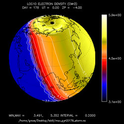
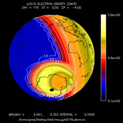
Brief Description: These simulation results show the electron density in the ionosphere at 150km. The top two movies depict results of simulations that use a model of the magnetosphere and solar EUV radiation levels typical for solar maximum during the northern hemisphere summer. The bottom movies were generated with the same conditions but with a simulated geomagnetic storm. Features such as the increase in ionoization on the day side, the auroral oval, and the expansion of the oval can be seen.

Time and Length Scale: Each movie represent one full day. The earth is represented to scale and all views are from the dawn side with sunlight coming in from the right. The northern hemisphere is viewed from a point at 40 degrees latitude while the southern hemisphere is viewed from a point at 45 degrees latitude.

Primary Author: Alan Burns and Stan Solomon, NSF Center for Integrated Space Weather Modeling

Cite Thus: A. G. and Solomon, S. C. . The package was developed by Ben Foster and applied by Zach Mullen.

Model and input files: These simulation results were generated using the TIEGCM model driven by an emperical magnetosphere. The F10.7 radio frequency flux is used as a proxy for EUV radiation levels that drive the ionospheric model. The magnetosphere model takes the polar cap potential as imput. Typical values for these parameters are used for solar minimum (not shown), solar maximum, and storm time.

Data Representation: The four links to avi's presented below show the electron density in the ionosphere at approximately 150 km. The color map is the log of electron density in particles per cm^3. All images are viewed from the dawn side: at 40 degrees North in the northern hemisphere, and 45 degrees South in the southern hemisphere. This was done to better view the auroral oval in the south. The sunlite side can be identified by its high ionization (yellow). The videos consist of 24 frames run at 5 fps showing 24 hours of time (UT 0:00-23:00, one rotation of the earth). The top images are a single day during the northern hemisphere summer and solar maximum. The bottom images are the same only a geomagnetic storm begins at before 1000 UT and ends before 2100 UT.

40 degrees North Quie	45 degrees South Quie
40 degrees North Stor	45 degrees South Stor

 

What event or situation was being simulated?: This is an idealized case. The effect of solar maximum relative to solar minimum is to increase the EUV radiation that drives the thermosphere and ionosphere. F10.7 radio frequency flux is used as a proxy for the EUV flux and represents an input to the thermosphere-ionosphere model. The polar cap potential is used as a driver for the emperical magnetosphere model. Appropriate values are used to drive the system for solar maximum, and then for a storm as an interplanetary coronal mass ejection stricks the magnetosphere..

Why was this run done?: The runs were part of a study to compare the difference between "ideal" solar minimum and solar maximum cases, and then compare the solar maximum case to the storm time case.

Notable Features: The dayside increase in ionization by over 2 orders of magnitude is clearly visible as well as the auroral oval. The offset of the magnetic poles from the rotational poles is also clearly visible as well as the mirroring between the north and south poles. Finally, during the storm, the sudden onset of the expansion of the auroral oval, and then the dramatic decrease at the end of the storm are due to the short recombination time of ions and electrons at the altitudes we are viewing. At higher altitudes the density is so low that recombination takes a much longer time. Thus at higher altitudes the affects of the storm can last for hours or even a day after the storm has ended.